# A tibble: 5 × 2
  Term                     Genes
  <chr>                    <chr>
1 phosphorylation          ACVRL1,FGF2,MAP2K1
2 vasculature development  CXCR4,RECK,EFNB2,PNPLA6,THY1,CAV1,CDH2,CDH5,ECSCR,HB…
3 blood vessel development CXCR4,RECK,PNPLA6,THY1,CAV1,CDH2,CDH5,ECSCR,HBEGF,AM…
4 cell adhesion            THY1,CDH2,CDH5
5 plasma membrane CXCR4,RECK,EFNB2,PNPLA6,THY1,CAV1,CDH2,CDH5,ECSCR,HB…R语言如何绘制富集弦图
前言
本篇是R包GOplot绘制富集弦图的教程,GOplot包的版本是V1.0.2,安装方式为 devtools::install_github(“wencke/wencke.github.io”),不是V1.0.2的版本会报错。
什么是富集弦图
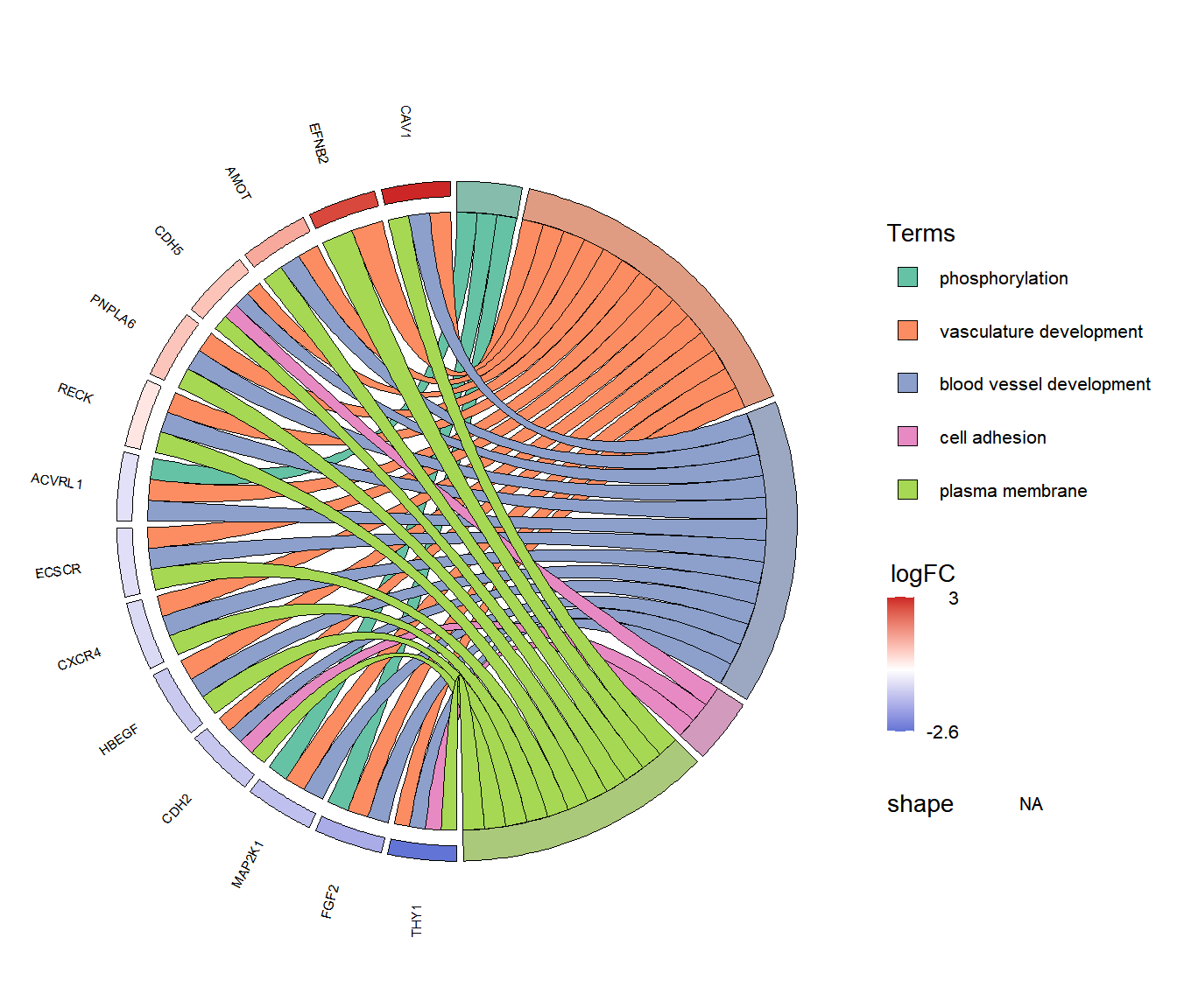
富集弦图:分别展示出每个Term富集到哪些基因以及这些基因的上下调情况。
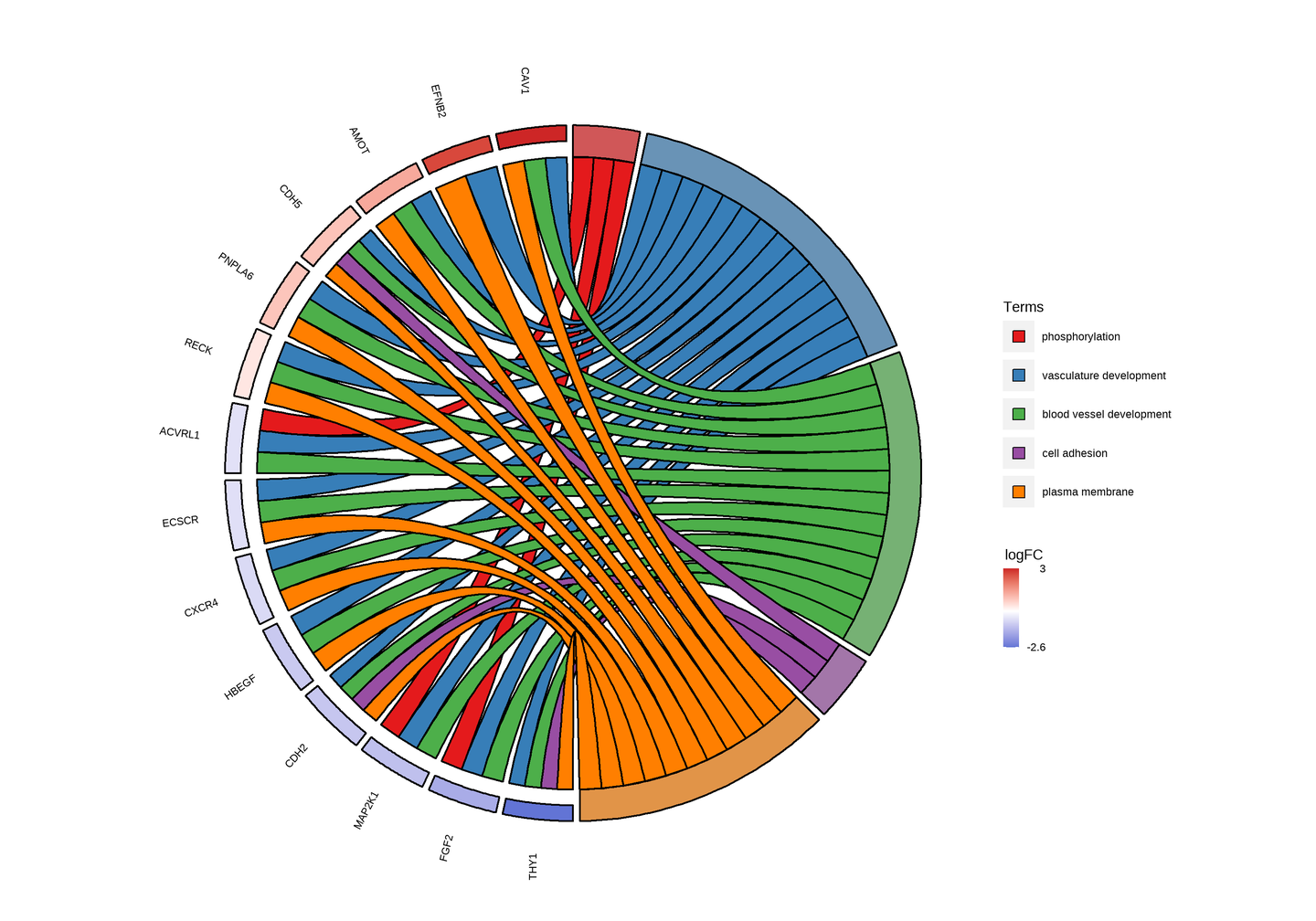
左侧为差异基因,颜色变化表示logFC从小到大的变化,红色为上调,蓝色为下调;右侧为富集结果的Term,两者相连表示基因富集到该Term中。
富集弦图一般显示3-10个通路较为合适,太多通路,会导致太过密集,反而看不清。
绘图前的数据准备
需要2个文件
每个通路对应哪些基因
包含2列数据,第1列为通路名称,第2列为每个通路对应的基因,基因之间用”,“或”, “或”|“分隔开。
demo数据可以从这下载:https://www.r2omics.cn/res/demodata/enrichChord/data.txt
每个基因对应的logFC(可选)
第一列为基因名称,第二列为logFC。注意基因要和第一个文件对应。空着的话,基因的方格会显示黑色。
demo数据可以从这下载:https://www.r2omics.cn/res/demodata/enrichChord/gene2FC.txt
# A tibble: 14 × 2
   Gene    logFC
   <chr>   <dbl>
 1 CXCR4  -0.653
 2 RECK    0.371
 3 EFNB2   2.65
 4 PNPLA6  0.870
 5 THY1   -2.56
 6 CAV1    3.69
 7 CDH2   -1.00
 8 CDH5    0.891
 9 ECSCR  -0.554
10 HBEGF  -0.957
11 AMOT    1.28
12 ACVRL1 -0.515
13 FGF2   -1.48
14 MAP2K1 -1.12
R语言如何绘制富集弦图
需要加载的程序
注意:GOplot包默认的效果感觉不是很好,字体重叠,且不圆,黑边太粗,图例只能在下面,所以我把源码改了改。运行正式的程序之前先把下面的代码加载了。适用于GOplot包的版本是V1.0.2,安装方式为 devtools::install_github(“wencke/wencke.github.io”),不是V1.0.2的版本会报错。
# 代码来源:https://www.r2omics.cn/
# 运行正式的程序之前先把下面的代码加载了
library(GOplot)
theme_blank <- theme(axis.line = element_blank(), axis.text.x = element_blank(),
                     axis.text.y = element_blank(), axis.ticks = element_blank(), axis.title.x = element_blank(),
                     axis.title.y = element_blank(), panel.background = element_blank(), panel.border = element_blank(),
                     panel.grid.major = element_blank(), panel.grid.minor = element_blank(), plot.background = element_blank())

check_chord <- function(mat, limit){

  if(all(colSums(mat) >= limit[2]) & all(rowSums(mat) >= limit[1])) return(mat)

  tmp <- mat[(rowSums(mat) >= limit[1]),]
  mat <- tmp[,(colSums(tmp) >= limit[2])]

  mat <- check_chord(mat, limit)
  return(mat)
}

# Bezier function for drawing ribbons
bezier <- function(data, process.col){
  x <- c()
  y <- c()
  Id <- c()
  sequ <- seq(0, 1, by = 0.01)
  N <- dim(data)[1]
  sN <- seq(1, N, by = 2)
  if (process.col[1] == '') col_rain <- grDevices::rainbow(N) else col_rain <- process.col
  for (n in sN){
    xval <- c(); xval2 <- c(); yval <- c(); yval2 <- c()
    for (t in sequ){
      xva <- (1 - t) * (1 - t) * data$x.start[n] + t * t * data$x.end[n]
      xval <- c(xval, xva)
      xva2 <- (1 - t) * (1 - t) * data$x.start[n + 1] + t * t * data$x.end[n + 1]
      xval2 <- c(xval2, xva2)
      yva <- (1 - t) * (1 - t) * data$y.start[n] + t * t * data$y.end[n]
      yval <- c(yval, yva)
      yva2 <- (1 - t) * (1 - t) * data$y.start[n + 1] + t * t * data$y.end[n + 1]
      yval2 <- c(yval2, yva2)
    }
    x <- c(x, xval, rev(xval2))
    y <- c(y, yval, rev(yval2))
    Id <- c(Id, rep(n, 2 * length(sequ)))
  }
  df <- data.frame(lx = x, ly = y, ID = Id)
  return(df)
}

GOCluster<-function(chord, process, metric, clust, clust.by, nlfc, lfc.col, lfc.min, lfc.max, lfc.space, lfc.width, term.col, term.space, term.width,process.label){
  x <- y <- xend <- yend <- width <- space <- logFC <- NULL
  if (missing(metric)) metric<-'euclidean'
  if (missing(clust)) clust<-'average'
  if (missing(clust.by)) clust.by<-'term'
  if (missing(nlfc)) nlfc <- 0
  if (missing(lfc.col)) lfc.col<-c('firebrick1','white','dodgerblue')
  if (missing(lfc.min)) lfc.min <- -3
  if (missing(lfc.max)) lfc.max <- 3
  if (missing(process.label)) process.label <- 11
  if (missing(lfc.space)) lfc.space <- (-0.5) else lfc.space <- lfc.space*(-1)
  if (missing(lfc.width)) lfc.width <- (-1.6) else lfc.width <- lfc.space-lfc.width-0.1
  if (missing(term.col)) term.col <- brewer.pal(length(process), 'Set3')
  if (missing(term.space)) term.space <- lfc.space + lfc.width else term.space <- term.space*(-1)
  if (missing(term.width)) term.width <- lfc.width + term.space else term.width <- term.width*(-1)+term.space


  if (clust.by == 'logFC') distance <- stats::dist(chord[,dim(chord)[2]], method=metric)
  if (clust.by == 'term') distance <- stats::dist(chord, method=metric)
  cluster <- stats::hclust(distance ,method=clust)
  dendr <- dendro_data(cluster)
  y_range <- range(dendr$segments$y)
  x_pos <- data.frame(x=dendr$label$x, label=as.character(dendr$label$label))
  chord <- as.data.frame(chord)
  chord$label <- as.character(rownames(chord))
  all <- merge(x_pos, chord, by='label')
  # print(all)
  all$label <- as.character(all$label)
  if (nlfc != 0){
    num <- ncol(all)-2-nlfc
    tmp <- seq(lfc.space, lfc.width, length = num)
    lfc <- data.frame(x=numeric(),width=numeric(),space=numeric(),logFC=numeric())
    for (l in 1:nlfc){
      tmp_df <- data.frame(x = all$x, width=tmp[l+1], space = tmp[l], logFC = all[,ncol(all)-nlfc+l])
      lfc<-rbind(lfc,tmp_df)
    }
  }else{
    lfc <- all[,c(2, dim(all)[2])]
    lfc$space <- lfc.space
    lfc$width <- lfc.width
  }
  term <- all[,c(2:(length(process)+2))]
  # print(dim(term)[1])
  color<-NULL;termx<-NULL;tspace<-NULL;twidth<-NULL
  for (row in 1:dim(term)[1]){
    idx <- which(term[row,-1] != 0)
    if(length(idx) != 0){
      termx<-c(termx,rep(term[row,1],length(idx)))
      color<-c(color,term.col[idx])
      tmp<-seq(term.space,term.width,length=length(idx)+1)
      tspace<-c(tspace,tmp[1:(length(tmp)-1)])
      twidth<-c(twidth,tmp[2:length(tmp)])
    }
  }
  tmp <- sapply(lfc$logFC, function(x) ifelse(x > lfc.max, lfc.max, x))
  logFC <- sapply(tmp, function(x) ifelse(x < lfc.min, lfc.min, x))
  lfc$logFC <- logFC
  term_rect <- data.frame(x = termx, width = twidth, space = tspace, col = color)
  # width_x = (max(all$x)-min(all$x))/nrow(all)
  # print(width_x)

  legend <- data.frame(x = 1:length(process),label = process)


  ggplot()+
    geom_segment(data=segment(dendr), aes(x=x, y=y, xend=xend, yend=yend))+
    geom_rect(data=lfc,aes(xmin=x-0.5,xmax=x+0.5,ymin=width,ymax=space,fill=logFC))+
    scale_fill_gradient2('logFC', space = 'Lab', low=lfc.col[3],mid=lfc.col[2],high=lfc.col[1],
                         guide=guide_colorbar(title.position='top',title.hjust=0.5,barwidth=1,barheight = 5,label.hjust = 1,label.vjust = 0.5,direction="vertical"),
                         # breaks = c(lfc.min,lfc.max),labels = c(lfc.min,lfc.max)
                         breaks=c(min(lfc$logFC),max(lfc$logFC)),labels=c(round(min(lfc$logFC),1),round(max(lfc$logFC),1))
    )+
    geom_rect(data=term_rect,aes(xmin=x-0.5,xmax=x+0.5,ymin=width,ymax=space),fill=term_rect$col)+
    # geom_rect(data=term_rect,aes(xmin=x-width_x-1,xmax=x+width_x+1,ymin=width,ymax=space),fill=term_rect$col)+
    geom_point(data=legend,aes(x=x,y=0.1,size=factor(label,levels=label),shape=NA))+
    guides(size=guide_legend("Terms",ncol=1,byrow=T,override.aes=list(shape=22,fill=term.col,size = 8),title.position="top",title.hjust = 0.5,order = 1))+
    coord_polar()+
    scale_y_reverse()+
    theme(legend.position='right',legend.text = element_text(size = process.label),legend.background = element_rect(fill='transparent'),legend.box='horizontal',legend.direction='horizontal')+
    theme_blank

}
# GOCluster_(chord = chord,process=process,clust.by = "logFC")
GOChord<-function(data, title, space, gene.order, gene.size, gene.space, nlfc = 1, lfc.col, lfc.min, lfc.max, ribbon.col, border.size, process.label, limit, scale.title,colorBar=T) {
  y <- id <- xpro <- ypro <- xgen <- ygen <- lx <- ly <- ID <- logFC <- NULL
  Ncol <- dim(data)[2]
  if (missing(title)) title <- ""
  if (missing(scale.title)) scale.title <- "logFC"
  if (missing(space)) space = 0
  if (missing(gene.order)) gene.order <- "none"
  if (missing(gene.size)) gene.size <- 3
  if (missing(gene.space)) gene.space <- 0.2
  if (missing(lfc.col)) lfc.col <- c("brown1", "azure", "cornflowerblue")
  if (missing(lfc.min)) lfc.min <- -3
  if (missing(lfc.max)) lfc.max <- 3
  if (missing(border.size)) border.size <- 0.5
  if (missing(process.label)) process.label <- 11
  if (missing(limit)) limit <- c(0, 0)
  if (gene.order == "logFC") data <- data[order(data[, Ncol], decreasing = T), ]
  if (gene.order == "alphabetical") data <- data[order(rownames(data)), ]
  if (sum(!is.na(match(colnames(data), "logFC"))) > 0) {
    if (nlfc == 1) {
      cdata <- check_chord(data[, 1 : (Ncol - 1)], limit)
      lfc <- sapply(rownames(cdata), function(x) data[match(x, rownames(data)), Ncol])
    } else {
      cdata <- check_chord(data[, 1 : (Ncol - nlfc)], limit)
      lfc <- sapply(rownames(cdata), function(x) data[, (Ncol - nlfc + 1)])
    }
  } else {
    cdata <- check_chord(data, limit)
    lfc <- 0
  }
  if (missing(ribbon.col)) colRib <- grDevices::rainbow(dim(cdata)[2]) else colRib <- ribbon.col
  nrib <- colSums(cdata)
  ngen <- rowSums(cdata)
  Ncol <- dim(cdata)[2]
  Nrow <- dim(cdata)[1]
  colRibb <- c()
  for (b in 1 : length(nrib)) colRibb <- c(colRibb, rep(colRib[b], 202 * nrib[b]))
  r1 <- 1
  r2 <- r1 + 0.1
  xmax <- c()
  x <- 0
  for (r in 1 : length(nrib)) {
    perc <- nrib[r] / sum(nrib)
    xmax <- c(xmax, (pi * perc) - space)
    if (length(x) <= Ncol - 1) x <- c(x, x[r] + pi * perc)
  }
  xp <- c()
  yp <- c()
  l <- 50
  for (s in 1 : Ncol) {
    xh <- seq(x[s], x[s] + xmax[s], length = l)
    xp <- c(xp, r1 * sin(x[s]), r1 * sin(xh), r1 * sin(x[s] + xmax[s]), r2 * sin(x[s] + xmax[s]), r2 * sin(rev(xh)), r2 * sin(x[s]))
    yp <- c(yp, r1 * cos(x[s]), r1 * cos(xh), r1 * cos(x[s] + xmax[s]), r2 * cos(x[s] + xmax[s]), r2 * cos(rev(xh)), r2 * cos(x[s]))
  }
  df_process <- data.frame(x = xp, y = yp, id = rep(c(1 : Ncol), each = 4 + 2 * l))
  xp <- c()
  yp <- c()
  logs <- NULL
  x2 <- seq(0 - space, -pi - (-pi / Nrow) - space, length = Nrow)
  xmax2 <- rep(-pi / Nrow + space, length = Nrow)
  for (s in 1 : Nrow) {
    xh <- seq(x2[s], x2[s] + xmax2[s], length = l)
    if (nlfc <= 1) {
      xp <- c(xp, (r1 + 0.05) * sin(x2[s]), (r1 + 0.05) * sin(xh), (r1 + 0.05) * sin(x2[s] + xmax2[s]), r2 * sin(x2[s] + xmax2[s]), r2 * sin(rev(xh)), r2 * sin(x2[s]))
      yp <- c(yp, (r1 + 0.05) * cos(x2[s]), (r1 + 0.05) * cos(xh), (r1 + 0.05) * cos(x2[s] + xmax2[s]), r2 * cos(x2[s] + xmax2[s]), r2 * cos(rev(xh)), r2 * cos(x2[s]))
    } else {
      tmp <- seq(r1, r2, length = nlfc + 1)
      for (t in 1 : nlfc) {
        logs <- c(logs, data[s, (dim(data)[2] + 1 - t)])
        xp <- c(xp, (tmp[t]) * sin(x2[s]), (tmp[t]) * sin(xh), (tmp[t]) * sin(x2[s] + xmax2[s]), tmp[t + 1] * sin(x2[s] + xmax2[s]), tmp[t + 1] * sin(rev(xh)), tmp[t + 1] * sin(x2[s]))
        yp <- c(yp, (tmp[t]) * cos(x2[s]), (tmp[t]) * cos(xh), (tmp[t]) * cos(x2[s] + xmax2[s]), tmp[t + 1] * cos(x2[s] + xmax2[s]), tmp[t + 1] * cos(rev(xh)), tmp[t + 1] * cos(x2[s]))
      }
    }
  }
  if (lfc[1] != 0) {
    if (nlfc == 1) {
      df_genes <- data.frame(x = xp, y = yp, id = rep(c(1 : Nrow), each = 4 + 2 * l), logFC = rep(lfc, each = 4 + 2 * l))
    } else {
      df_genes <- data.frame(x = xp, y = yp, id = rep(c(1 : (nlfc * Nrow)), each = 4 + 2 * l), logFC = rep(logs, each = 4 + 2 * l))
    }
  } else {
    df_genes <- data.frame(x = xp, y = yp, id = rep(c(1 : Nrow), each = 4 + 2 * l))
  }
  aseq <- seq(0, 180, length = length(x2))
  angle <- c()
  for (o in aseq) if ((o + 270) <= 360) angle <- c(angle, o + 270) else angle <- c(angle, o - 90)
  df_texg <- data.frame(xgen = (r1 + gene.space) * sin(x2 + xmax2 / 2), ygen = (r1 + gene.space) * cos(x2 + xmax2 / 2), labels = rownames(cdata), angle = angle)
  df_texp <- data.frame(xpro = (r1 + 0.15) * sin(x + xmax / 2), ypro = (r1 + 0.15) * cos(x + xmax / 2), labels = colnames(cdata), stringsAsFactors = FALSE)
  cols <- rep(colRib, each = 4 + 2 * l)
  x.end <- c()
  y.end <- c()
  processID <- c()
  for (gs in 1 : length(x2)) {
    val <- seq(x2[gs], x2[gs] + xmax2[gs], length = ngen[gs] + 1)
    pros <- which((cdata[gs, ] != 0) == T)
    for (v in 1 : (length(val) - 1)) {
      x.end <- c(x.end, sin(val[v]), sin(val[v + 1]))
      y.end <- c(y.end, cos(val[v]), cos(val[v + 1]))
      processID <- c(processID, rep(pros[v], 2))
    }
  }
  df_bezier <- data.frame(x.end = x.end, y.end = y.end, processID = processID)
  df_bezier <- df_bezier[order(df_bezier$processID, -df_bezier$y.end), ]
  x.start <- c()
  y.start <- c()
  for (rs in 1 : length(x)) {
    val <- seq(x[rs], x[rs] + xmax[rs], length = nrib[rs] + 1)
    for (v in 1 : (length(val) - 1)) {
      x.start <- c(x.start, sin(val[v]), sin(val[v + 1]))
      y.start <- c(y.start, cos(val[v]), cos(val[v + 1]))
    }
  }
  df_bezier$x.start <- x.start
  df_bezier$y.start <- y.start
  df_path <- bezier(df_bezier, colRib)
  if (length(df_genes$logFC) != 0) {
    tmp <- sapply(df_genes$logFC, function(x) ifelse(x > lfc.max, lfc.max, x))
    logFC <- sapply(tmp, function(x) ifelse(x < lfc.min, lfc.min, x))
    df_genes$logFC <- logFC
  }
  g <- ggplot() +
    geom_polygon(data = df_process, aes(x, y, group = id), fill = "gray70", inherit.aes = F, color = "black",size = border.size) +
    geom_polygon(data = df_process, aes(x, y, group = id), fill = cols, inherit.aes = F, alpha = 0.6, color = "black",size = border.size) +
    geom_point(aes(x = xpro, y = ypro, size = factor(labels, levels = labels), shape = NA), data = df_texp) +
    guides(size = guide_legend("Terms",ncol = 1, byrow = T, override.aes = list(shape = 22, fill = unique(cols), size = process.label/2),title.position = "top",title.hjust = 0,order = 1)) +
    theme(legend.text = element_text(size = process.label)) +
    geom_text(aes(xgen, ygen, label = labels, angle = angle), data = df_texg, size = gene.size) +
    geom_polygon(aes(x = lx, y = ly, group = ID), data = df_path, fill = colRibb, color = "black", size = border.size, inherit.aes = F) +
    labs(title = title) + coord_fixed()+
    theme_blank
  if (colorBar) {
    g + geom_polygon(data = df_genes, aes(x, y, group = id, fill = logFC), inherit.aes = F, color = "black",size = border.size) +
      scale_fill_gradient2(scale.title, space = "Lab", low = lfc.col[3], mid = lfc.col[2], high = lfc.col[1],
                           guide = guide_colorbar(title.position = "top",title.hjust=0.5,barwidth=process.label/10,barheight = process.label/2,label.hjust = 1,label.vjust = 0.5,direction="vertical"),
                           # breaks = c(lfc.min,lfc.max),labels = c(lfc.min,lfc.max)
                           breaks = c(min(df_genes$logFC), max(df_genes$logFC)), labels = c(round(min(df_genes$logFC),1), round(max(df_genes$logFC),1))
      ) +
      theme(legend.position = "right",legend.title = element_text(size = process.label*4/3),legend.text = element_text(size = process.label), legend.background = element_rect(fill = "white"), legend.direction = "horizontal") # ,legend.box = "horizontal"
  } else {

    g + geom_polygon(data = df_genes, aes(x, y, group = id), fill = "skyblue", inherit.aes = F, color = "black",size = border.size) #+
    #theme(legend.position = "bottom",legend.text = element_text(size = process.label), legend.background = element_rect(fill = "white"), legend.box = "horizontal", legend.direction = "horizontal")

  }

}
正式程序
# 代码来源:https://www.r2omics.cn/
# 转载所需要的包
library(tidyverse)    # 用于数据处理
library(GOplot)       # 用于绘图  安装方式 devtools::install_github("wencke/wencke.github.io")
library(RColorBrewer) # 颜色

# 读取数据
dfTerm =  read.delim("https://www.r2omics.cn/res/demodata/enrichChord/data.txt")
dfFC =  read.delim("https://www.r2omics.cn/res/demodata/enrichChord/gene2FC.txt")


# 整理数据
dfClean = dfTerm %>%
  separate_rows(Genes,sep = ",") %>%
  left_join(dfFC,by=c("Genes"="Gene"))

dfPlot = chord_dat(data.frame(dfClean),  process=unique(dfClean$Term))

# 绘图
GOChord(dfPlot,
        border.size=0.1,           # 线条黑边的粗细
        space = 0.02,              # 基因方格之间的空隙
        gene.order = "logFC",      #  基因的排序方式,可以按照"logFC", "alphabetical", "none",
        gene.space = 0.3,          # 基因标签离图案的距离
        gene.size = 2,             # 基因标签的大小
        lfc.col=c('firebrick3', 'white','royalblue3'), # logFC图例的颜色
        ribbon.col=brewer.pal(ncol(dfPlot)-1, "Set2"),   # 条带颜色设置
        process.label = 8          # 图例标签的大小
)